Huge amounts of climate data is distributed as open access. However, in many cases the data formats and required tools are complicated to use and amount of data can exceed users capacity. On the other hand, online tools for data visualization might be limited in terms of functionality.
Climate Data Tools is a collection of codes developed to utilize climate data from original data sources, with possibilities of basic processing and visualization, together with high-level of personalization and development opportunities. We provide tools to access original data from several sources, including CMIP6, NASA, EBAS, …
Don’t want to download data to your computer? Use MyBinder!

https://mybinder.org/v2/gh/ClimComp/ClimateDataTools/HEAD

Mybinder is a service for creating and sharing computational environments. With it you can initialize an appropriate environment for our codes and run them without downloading anything. It has some limitations, namely RAM and session time limits of 2GB and 10 minutes of inactivity respectively. This means that not all longer and more complex codes will work there, but if you want to access and use simpler examples it is very easy to use just by clicking the link.
How to use the codes on my computer? Install Conda!
Conda is a package and environment manager that can be very useful when you need multiple packages with many dependencies. It makes downloading specific versions of packages easier and allows to share full environments with configuration files so there is no need to install every package separately.
Setting up a conda environment:
- Download Anaconda and set it up to PATH
- Download Visual Studio Code or a similar editor
- Open the editor, set up Python and Jupyter extensions if needed (at least in Visual Studio Code)
- Visit our GitHub repository, click “Code” -> “Download ZIP”
- Unzip the directory, navigate to it in Anaconda Prompt (cd your/path/to/directory)
- Check what environment file is needed, then create a new environment with the said .yml file (ALTERNATIVE: after 7., see the list of required packages in the file and download them manually)
- Type “code” into the Anaconda Prompt to start Visual Studio Code
- Open the file of interest, check that the right environment is active (upper right corner in Visual Studio Code)
- Program can now be run
About CMIP6 data:

Coupled Model Intercomparison Project 6 (CMIP6) is a framework enabling a systematic analysis of different climate models. It consists of both historical simulations and future scenarios. The main ways of accessing CMIP6 data are through ESGF and Pangeo. ESGF stores all the available data while only some of the data is available in Pangeo’s cloud storage. However, ESGF’s data isn’t always as easily approachable as Pangeo’s and one dataset can be divided into several files.
The following are examples of running scripts from Climate Data Tools. Follow the link to see the code in GitHub, and run the code in cloud (e.g. MyBinder) or on your own computer.
Pangeo: Simple One Dataset Example Using Intake-Esm


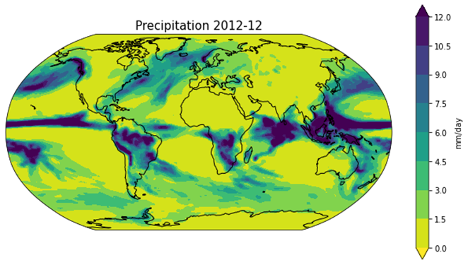
Pangeo also offers the CMIP6 data in so-called intake-esm catalogs. This example shows how to search for data from Pangeo using intake-esm and how to visualize a dataset with basic maps.
GitHub: https://github.com/ClimComp/ClimateDataTools/blob/main/Pangeo/simple_tas_example_(intake-esm).ipynb
Pangeo: One CMIP6 Dataset from Google Cloud Storage in Zarr-Format

CMIP6 data is stored Pangeo’s Google Cloud Storage as zarr objects. Zarr datastores on the other hand are saved into CSV-file. This example goes through how to access the data in Google Cloud Storage and how to visualize a dataset with maps.
GitHub: https://github.com/ClimComp/ClimateDataTools/blob/main/Pangeo/simple_pr_example_(zarr-format).ipynb
Pangeo: Timeseries of Global Temperature and Precipitation Anomalies

In this example we search Pangeo’s intake-esm catalogue for models that have both historical and ssp119-scenario datasets and calculate and plot time series of annual global means.
GitHub: https://github.com/ClimComp/ClimateDataTools/blob/main/Pangeo/tas_and_pr_timeseries_2.ipynb
Pangeo: Near Surface Air Temperature Anomaly Animation

This program searches for historical and ssp585 data from Google Cloud Storage, calculates the average of 20 different models and creates a video of temperature anomaly (relative to 1850-1900).
GitHub: https://github.com/ClimComp/ClimateDataTools/blob/main/Pangeo/AnomalyAnimation/tas_animation.ipynb
Pangeo: Near Surface Air Temperature Anomaly Animation of Two Scenarios

This program searches for historical, ssp119 and ssp585 data from Google Cloud Storage and calculates the average of 20 different models. Then it animates a figure with two maps and a time series of global averages.
Pangeo: Anomalies of the Arctic example

This program is used to plot anomalies of different variables in the Arctic area. Some interesting variables are, for example, temperature near the surface, sea ice thickness and cloud cover. GitHub: https://github.com/ClimComp/ClimateDataTools/blob/main/Pangeo/arctic_anomalies.ipynb
ESGF: Simple One Dataset Example


This example goes through how to access data from Earth System Grid Federation (ESGF) and visualize the data with simple plots. ESGF stores the datasets as netCDF files, but in many cases one dataset can be divided into multiple files.
GitHub: https://github.com/ClimComp/ClimateDataTools/blob/main/ESGF/ESGF_tas_example.ipynb
ESGF: Aerosol time series example


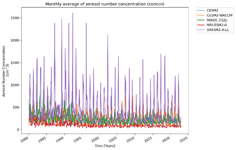
This program is used to download and analyze different aerosol variables in a certain location using ESGF’s CMIP6 data. It plots the monthly data from each model as well as the yearly averages with a trendline.
GitHub: https://github.com/ClimComp/ClimateDataTools/blob/main/ESGF/ESGF_aersosol_timeseries.ipynb
Climate Data Store API example


This example goes through retrieving ERA5 Monthly Averaged Data with an API request from CDS and plots two variables from the dataset.
GitHub: https://github.com/ClimComp/ClimateDataTools/blob/main/C3S-ClimateDataStore/CDS-API.ipynb
NSIDC: Sea ice concentration example


This program demonstrates the usage of sea ice data downloaded from the National Snow and Ice Data Center via FTP to create an animation of yearly sea ice concentration in the Arctic.
GitHub: https://github.com/ClimComp/ClimateDataTools/blob/main/NSIDC/NSIDC_Sea_Ice.ipynb
Shapefile examples


This program demonstrates the usage of shapefiles. The first part uses heatwave shapefiles from the European Environment Agency and the second permafrost, tree line and subsea extent of permafrost shapefiles from the National Snow and Ice Data Center downloaded via FTP.
GitHub: https://github.com/ClimComp/ClimateDataTools/blob/main/NSIDC/Shapefile_examples.ipynb
NASA: Nitrogen Dioxide CSV example

This program reads satellite data from NASA and converts the CSV file into an animation.
GitHub: https://github.com/ClimComp/ClimateDataTools/blob/main/NASA/Earth_Observatory_NO2.ipynb
ESA: Ocean Color example

This program creates an animation from ESA’s chlorophyll satellite data with a chosen resolution.
GitHub: https://github.com/ClimComp/ClimateDataTools/blob/main/ESA/ESA_Ocean_Color.ipynb
EBAS CCN example

This example illustrates the usage of EBAS data portal in retrieving aerosol data and plotting it.
GitHub: https://github.com/ClimComp/ClimateDataTools/blob/main/EBAS/EBAS_CCN.ipynb
Tools and reports
Panoply is a downloadable tool for visualizing geo-referenced data in netCDF, GRIB and other formats. You can use data from your disk or remotely through OpenDAP.
Climate Data Operators (CDO) is a collection of operators used to manipulate climate data in netCDF, GRIB and other formats. It is most often used from command line but there is also an interface available for Python and Ruby.
CDS Toolbox is one of the options to visualize data from CDS. The toolbox itself contains multiple ready-made examples you can use as your starting point, but C3S also offers plenty of other instructions to the use of the toolbox such as tutorials, how-to-guides and learning bundles.
Assessment Report 6 (AR6) is a comprehensive report on the causes and effects of climate change. It offers an in-depth look into the physical background behind climate change, its impact, adaptation and mitigation. It’s divided into 3 separate sections which can be found following the link above.
Special reports handle a specific topic, such as changes in oceanic and frozen environments caused by climate change.
Links:
ClimComp: https://blogs.helsinki.fi/climatecompetencies/
GitHub: https://github.com/ClimComp/ClimateDataTools
ClimComp has been funded by Research Council of Finland (2021–2024)